제목: Deep Residual Learning for image Recognition

학회: IEEE Conference on Computer Vision and Pattern Recognition

게재: 2016년


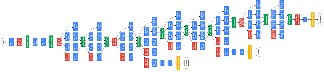
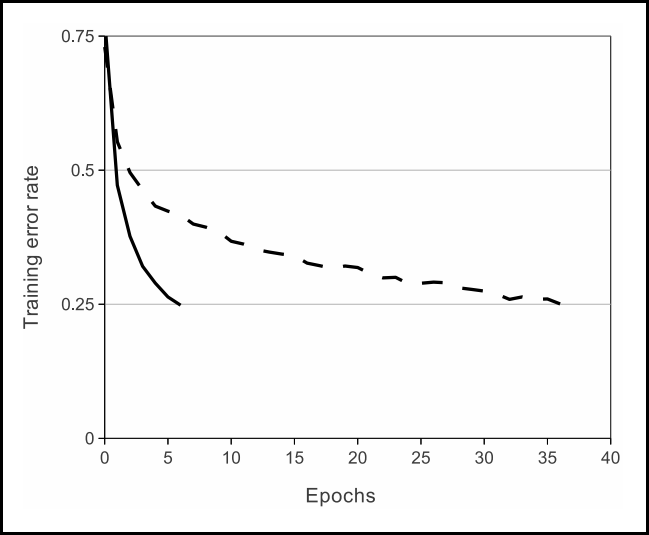
컴퓨터 비전에서 높은 이미지 인식 능력 모델의 발전은 AlexNet → VGGNet → GoogLeNet → ResNet 순으로 이뤄진다. 이러한 높은 인식 능력의 배경에는 네트워크의 깊이를 늘림으로써 high level feature부터 low level feature를 효율적으로 추출할 수 있기 때문이다. 대개 네트워크의 깊이를 늘림으로써 모델의 성능이 늘어난다. 하지만 반드시 그렇지는 않다. 아래 그래프가 이를 뒷받침 한다.


Training error & Test error on CIFAR-10 of "plain" network (no residual network)


위 그래프를 보면 상대적으로 더 깊은 네트워크가 training error가 더 높다. 즉 성능이 더 낮아진다. 왜 이렇게 낮아질까? 네트워크 깊이를 늘리는 데 있어 한계가 있기 때문이다. 그리고 그 한계란 gradient vanishing 문제를 말한다. 이는 레이어가 깊을수록 역전파를 하는 과정에서 미분 값이 줄어들기 때문에 앞단 레이어는 영향을 거의 받지 못하기 때문이다. 이 문제를 해결하기 위해 ResNet이 만들어졌다. 즉 ResNet은 gradient vanishing 문제를 해결하는 모델인 것이다. 그 핵심 방법은 아래 그림 오른쪽과 같이 residual network를 사용하는 것이다.


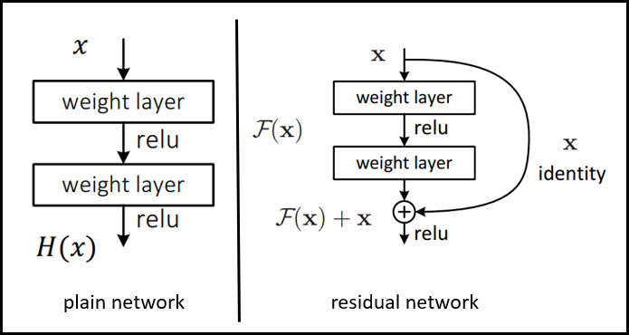
residual network는 앞단 레이어의 출력값이 입력으로 들어온 x를 feed forward 한 값에 다시 x를 더해준다. 이게 왜 효과가 있을까? 왼쪽 일반 신경망과의 학습 방식이 다르기 때문이다. 일반 신경망은 입력 $x$를 통해 출력 $H(x)$를 얻는 $H(x) = x$다. 반면 오른쪽 residual network는 $H(x) = F(x) + x$가 된다. 중간에 $F(x)$가 추가된 것이다. 이 때 이 추가된 $F(x)$를 0이 되도록 학습한다면 일반 신경망인 $H(x) = x$와 같아진다. 하지만 이렇게 둘러온다면 하나의 큰 장점이 있다. 일반 신경망처럼 역전파가 진행될 때 $H(x) = x$에서 미분하는 것과 달리 residual network를 이용해 미분하게 되면 $H'(x) = F'(x) + 1$이 된다. 즉 1도 남기 때문에 기울기가 0에 수렴하여 소실되지 않고 역전파가 끝까지 진행될 수 있는 것이다.


이해가 안될 경우를 대비해 조금 더 설명하면, $H(x) = F(x) +x$을 이항하면 $F(x) = H(x) - x$가 된다. 이 때 $F(x)$를 0에 근사하게 만든다면 $H(x) - x$도 0에 근사하게 된다. 다시 이항하면 기존 신경망과 같이 $H(x) = x$의 형태가 된다. 양쪽 모두 역전파로 인해 미분되어 0에 근사하게 되면 기울기 소실 문제가 발생하는 것이다. 참고로 $H(x) - x$을 residual이라 부르며, residual network에선 기존 신경망의 학습 목적인 $H(x)$를 최소화 해주는 것이 아니라 $F(x)$를 최소화 시켜주는 것이다. $F(x) = H(x) - x$이므로.


ResNet에서는 residual network를 아래 두 가지 방식을 사용해 구현했다. 첫 번째는 바로 위 그림과 마찬가지로 단순한 구조를 사용하는 Identity 방식과, 두 번째는 1x1 convolution 연산을 통해 차원을 스케일링 해주는 Projection 방식이다. 


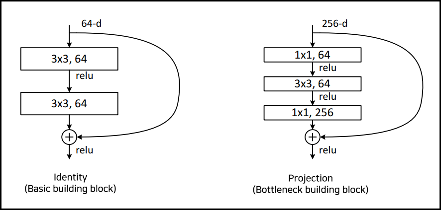
기존의 Identity 방식에 더해 Projection 방식이 더해진 이유는 입력/출력 차원이 다를 때 스케일링 해주기 위함이다.  또 Projection 방식은 네트워크를 깊게 만들어줄 때 학습 시간을 줄이기 위해 사용하는데, 위 두 구조가 비슷한 시간 복잡도를 갖기 때문이라고 한다.


다시 돌아와 이러한 residual network 구조를 사용하는 것이 ResNet 이해의 핵심이다. 이렇게 residual network를 모델 레이어로 쌓으면 다음과 같은 성능 증가를 가져오게 된다.


가는 선: training error / 굵은 선: validation error


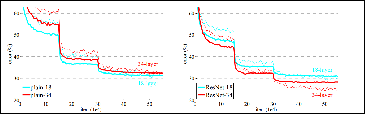
좌측의 residual network를 적용하지 않은 plain network를 살펴보면 레이어를 깊게 해줄수록 성능이 오히려 떨어지게 된다. 반면 residual network를 모델에 적용하게 되면 레이어가 깊더라도 error rate가 떨어져 성능이 더 좋아지는 것을 확인할 수 있다. 


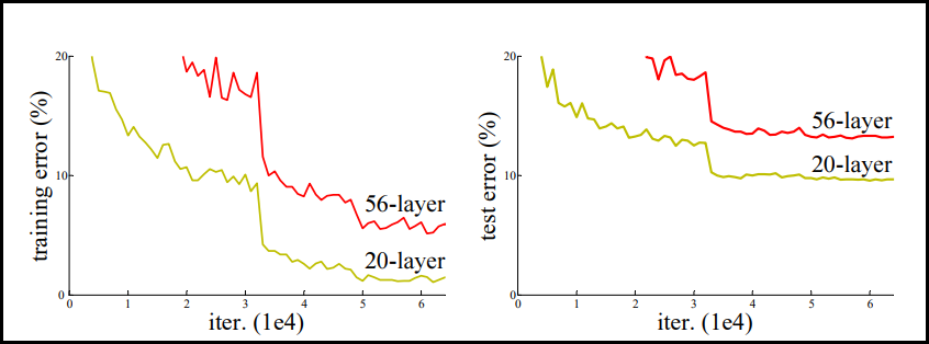
그렇다면 더욱 더 residual network를 쌓게 되면 어떤 결과가 나올까? 아래를 보자. 참고로 ResNet에서 50개의 layer가 넘어가는 모델들은 Projection 방법 (Bottleneck building block)을 사용하여 만든 모델이다. 반대로 50개 미만은 Identity 방법 (Basic building block)으로 만들었다.


model performance comparison on CIFAR-10 datasets


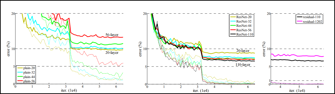
좌측 residual network를 적용하지 않은 plain network의 경우에는 레이어가 깊어질수록 성능이 계속 떨어지는 것을 볼 수 있다. 반면 가운데 그래프처럼 ResNet을 적용하면 error율이 아닐 때 보다 더 감소한 것을 볼 수 있다. 또한 110개의 네트워크를 쌓더라도 성능이 증가하는 것을 볼 수 있다. 다만 우측 그래프처럼 residual network를 1202개까지 쌓게 되면 오히려 110개를 쌓았을 때 보다 성능이 좋지 않다. 하지만 이를 두고 1202개 가량을 쌓았을 때가 ResNet의 한계라고 해석할 수 없다. 그 이유는 CIFAR-10 데이터셋만으로는 불충분해 overfitting 되었을 가능성이 있기 때문이고, 또 ResNet 논문 저자들은 그 어떤 Dropout과 같은 Regularization을 적용하지 않았다고 말했다. 따라서 강력한 Regularization을 적용한다면 성능 향상의 여지가 있는 것이다.


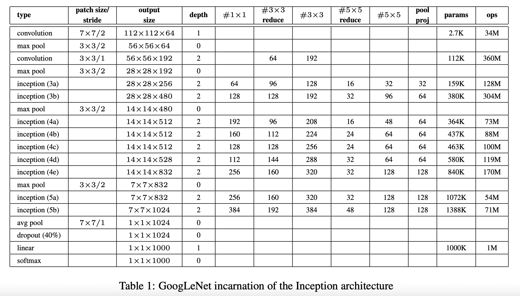
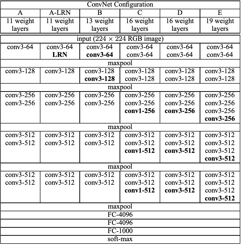
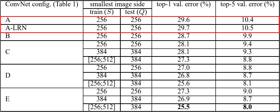
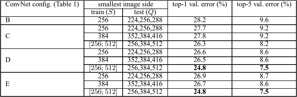
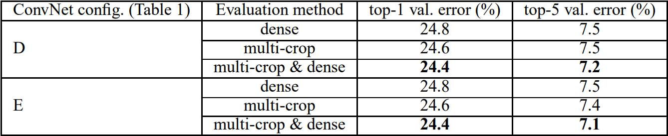
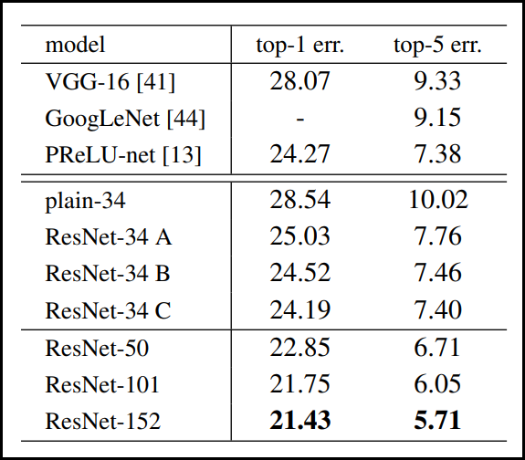
마지막으로, ResNet 모델의 개선 여지가 있음에도 불구하고 아래 표와 같이 이전에 나온 VGGNet과 GoogLeNet 모델보다도 높은 성능을 보였다. 


Error rate on ImageNet validation


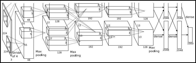
ResNet을 구현하기 위해 먼저 가장 핵심인 ResNet 모델 아키텍처를 살펴보면 다음과 같다.


하나의 max-pool 레이어와, 하나의 average-pool 레이어를 제외하고 모두 convolution 레이어로 구성되어 있다. 또 18, 34 layer는 레이어 구조상 Basic Building Block을 사용하며 50, 101, 152 layer는 Bottleneck Building Block을 사용한다. 


그리고 논문에서 구현에 적용되었던 augmentation 기법과 레이어 특이 사항, 하이퍼파라미터 값을 정리하면 다음과 같다.


1. Augmentation

  • 이미지를 스케일 별 augmentation을 위해 이미지 사이즈를 256~480 범위에서 랜덤 샘플링 진행
  • 픽셀별 mean substracted을 진행하고, 224x224 이미지에 crop을 랜덤 샘플링 수행하거나 수평 플립을 적용한 이미지에서 crop을 랜덤 샘플링함
  • color augmentation을 사용함


2. Layer

  • Batch Normalization 적용 (convolution 이후, activation function 이전)
  • weight initialization 진행
  • Dropout 미사용
  • residual network에서 차원이 증가한다면 아래 두 가지 방식 적용
    1. 제로 패딩으로 차원 증가에 대응: 추가적인 파라미터 없어 좋음
    2. 1x1 convolution으로 차원 스케일링 해준 뒤 다시 원래 차원으로 스케일링 진행 


3. Hyper-parameter

  • 옵티마이저: SGD 사용
  • 배치 사이즈: 256
  • weight decay: 0.0001, momentum: 0.9
  • 학습율: 0.1로 시작해서 validation error가 줄지 않으면 x10씩 줄여나감.
  • $60\times 10^4$ iteration까지 진행되었음


ResNet 구현을 위해 가장 먼저 핵심이 되는 Identity 방식의 Basic building block을 만들어준다. 


import torch
from torch import Tensor
import torch.nn as nn


class BasicBlock(nn.Module):
    expansion_factor = 1
    def __init__(self, in_channels: int, out_channels: int, stride: int = 1):
        super(BasicBlock, self).__init__()
        self.conv1 = nn.Conv2d(in_channels, out_channels, kernel_size=3, stride=stride, padding=1, bias=False)
        self.bn1 = nn.BatchNorm2d(out_channels)
        self.relu1 = nn.ReLU()

        self.conv2 = nn.Conv2d(out_channels, out_channels, kernel_size=3, stride=1, padding=1, bias=False)
        self.bn2 = nn.BatchNorm2d(out_channels)

        self.relu2 = nn.ReLU()
        self.residual = nn.Sequential()
        if stride != 1 or in_channels != out_channels * self.expansion_factor:
            self.residual = nn.Sequential(
                nn.Conv2d(in_channels, out_channels*self.expansion_factor, kernel_size=1, stride=stride, bias=False),
                nn.BatchNorm2d(out_channels*self.expansion_factor))
                
    def forward(self, x: Tensor) -> Tensor:
        out = x
        x = self.conv1(x)
        x = self.bn1(x)
        x = self.relu1(x)

        x = self.conv2(x)
        x = self.bn2(x)
        x += self.residual(out)
        x = self.relu2(x)
        return x


다음으로 또 다른 구조인 Projection 방식의 Bottleneck building block을 만들어 준다.


class BottleNeck(nn.Module):
    expansion_factor = 4
    def __init__(self, in_channels: int, out_channels: int, stride: int = 1):
        super(BottleNeck, self).__init__()

        self.conv1 = nn.Conv2d(in_channels, out_channels, kernel_size=1, stride=1, bias=False)
        self.bn1 = nn.BatchNorm2d(out_channels)
        self.relu1 = nn.ReLU()
        
        self.conv2 = nn.Conv2d(out_channels, out_channels, kernel_size=3, stride=stride, padding=1, bias=False)
        self.bn2 = nn.BatchNorm2d(out_channels)
        self.relu2 = nn.ReLU()
        
        self.conv3 = nn.Conv2d(out_channels, out_channels * self.expansion_factor, kernel_size=1, stride=1, bias=False)
        self.bn3 = nn.BatchNorm2d(out_channels*self.expansion_factor)
        
        self.relu3 = nn.ReLU()
        self.residual = nn.Sequential()
        if stride != 1 or in_channels != out_channels * self.expansion_factor:
            self.residual = nn.Sequential(
                nn.Conv2d(in_channels, out_channels*self.expansion_factor, kernel_size=1, stride=stride, bias=False),
                nn.BatchNorm2d(out_channels*self.expansion_factor))
        
    def forward(self, x:Tensor) -> Tensor:
        out = x
        x = self.conv1(x)
        x = self.bn1(x)
        x = self.relu1(x)

        x = self.conv2(x)
        x = self.bn2(x)
        x = self.relu2(x)
        
        x = self.conv3(x)
        x = self.bn3(x)
        
        x += self.residual(out)
        x = self.relu3(x)
        return x


위 두 구조에 따라 ResNet을 구성할 수 있도록 모델을 구성해준다.

class ResNet(nn.Module):
    def __init__(self, block, num_blocks, num_classes=10):
        super(ResNet, self).__init__()
        self.in_channels = 64
        self.conv1 = nn.Sequential(
            nn.Conv2d(in_channels=3, out_channels=64, kernel_size=7, stride=2, padding=3, bias=False),
            nn.BatchNorm2d(num_features=64),
            nn.ReLU(),
            nn.MaxPool2d(kernel_size=3, stride=2, padding=1))

        self.conv2 = self._make_layer(block, 64, num_blocks[0], stride=1)
        self.conv3 = self._make_layer(block, 128, num_blocks[1], stride=2)
        self.conv4 = self._make_layer(block, 256, num_blocks[2], stride=2)
        self.conv5 = self._make_layer(block, 512, num_blocks[3], stride=2)
        self.avgpool = nn.AdaptiveAvgPool2d(output_size=(1, 1))
        self.fc = nn.Linear(512 * block.expansion_factor, num_classes)

        self._init_layer()

    def _make_layer(self, block, out_channels, num_blocks, stride):
        strides = [stride] + [1] * (num_blocks-1)
        layers = []
        for stride in strides:
            layers.append(block(self.in_channels, out_channels, stride))
            self.in_channels = out_channels * block.expansion_factor
        return nn.Sequential(*layers)

    def _init_layer(self):
        for m in self.modules():
            if isinstance(m, nn.Conv2d):
                nn.init.kaiming_normal_(m.weight, mode='fan_out', nonlinearity='relu')
            elif isinstance(m, (nn.BatchNorm2d, nn.GroupNorm)):
                nn.init.constant_(m.weight, 1)
                nn.init.constant_(m.bias, 0)

    def forward(self, x: Tensor) -> Tensor:
        x = self.conv1(x)
        x = self.conv2(x)
        x = self.conv3(x)
        x = self.conv4(x)
        x = self.conv5(x)
        
        x = self.avgpool(x)
        x = torch.flatten(x, 1)
        x = self.fc(x)
        return x


ResNet 아키텍처에 표시된 레이어의 개수를 맞춰준 모델을 반환하는 클래스를 정의한다. 

class Model:
    def resnet18(self):
        return ResNet(BasicBlock, [2, 2, 2, 2])

    def resnet34(self):
        return ResNet(BasicBlock, [3, 4, 6, 3])

    def resnet50(self):
        return ResNet(BottleNeck, [3, 4, 6, 3])

    def resnet101(self):
        return ResNet(BottleNeck, [3, 4, 23, 3])

    def resnet152(self):
        return ResNet(BottleNeck, [3, 8, 36, 3])


마지막으로 간단한 테스트를 위해 모델을 불러오고 랜덤 생성한 데이터를 넣어주고 결과를 확인한다.

model = Model().resnet152()
y = model(torch.randn(1, 3, 224, 224))
print (y.size()) # torch.Size([1, 10])


데이터셋으로 직접 학습 시켜보고자 한다면 train 코드는 아래 링크에 함께 구비해두었다.


전체 코드: https://github.com/roytravel/paper-implementation/tree/master/resnet


Reference

[1] https://github.com/weiaicunzai/pytorch-cifar100/blob/master/models/resnet.py

[2] https://github.com/kuangliu/pytorch-cifar/blob/master/models/resnet.py

[3] https://github.com/pytorch/vision/blob/main/torchvision/models/resnet.py


논문: Going Deeper with convolutions
게재: 2015년
학회: CVPR

GoogLeNet이란?

GoogLeNet은 한 마디로 네트워크의 depth와 width를 늘리면서도 내부적으로 inception 모듈을 활용해 computational efficiency를 확보한 모델이다. 이전에 나온 VGGNet이 깊은 네트워크로 AlexNet보다 높은 성능을 얻었지만, 반면 파라미터 측면에서 효율적이지 못하다는점을 보완하기 위해 만들어졌다.


CNN 아키텍처와 GoogLeNet

2010년 초/중반 CNN 아키텍처를 활용해 높은 이미지 인식 능력을 선보인 모델은 AlexNet (2012) → VGGNet (2014) → GoogLeNet (2014) → ResNet (2015) → ... 순으로 계보가 이어진다. 이 모델들은 네트워크의 depth와 width를 늘리면서 성능 향상이 이루어지는 것을 보며 점점 depth와 width를 늘려갔다. 하지만 이렇게 네트워크가 커지면서 두 가지 문제점이 발생했다. 첫 번째는 많은 파라미터가 있지만 이를 학습시킬 충분한 데이터가 없다면 오버피팅이 발생하는 것이고, 두 번째는 computational resource는 늘 제한적이기에 비용이 많이 발생하거나 낭비될 수 있다는 점이다. GoogLeNet은 이러한 문제점을 해결하기 위해 fully-connected layer의 neuron 수를 줄이거나 convolution layer의 내부 또한 줄여 상대적으로 sparse한 network를 만들고자 만들어졌다. 결과적으로 GoogLeNet은 가장 초반에 나온 AlexNet보다도 파라미터수가 12배 더 적지만 더 높은 성능을 보이는 것이 특징이다. 결과적으로 GoogLeNet은 ILSVRC 2014에서 classification과 detection 트랙에서 SOTA를 달성했다.


Inception: GoogLeNet 성능의 핵심

파라미터 효율적이면서도 높은 성능을 낼 수 있는 GoogLeNet 아키텍처의 핵심은 내부 Inception 모듈의 영향이다. Inception 모듈을 보기전 먼저 GoogLeNet 아키텍처를 살펴보면 다음과 같다.


왼쪽(아래)에서 출발하여 오른쪽(위)으로 점점 깊어진다. Inception 모듈은 위 GoogLeNet 네트워크에서 사용되는 부분 네트워크에 해당한다. 그 부분 구조는 아래와 같다. 두 가지 버전이 있다.

두 버전 모두 이미지 feature를 효율적으로 추출하기 위해 공통적으로 1x1, 3x3, 5x5 필터 크기를 갖는 convolution 연산을 수행한다. 이렇게 이미지의 다양한 영역을 볼 수 있도록 서로 다른 크기의 필터를 사용함으로써 앙상블하는 효과를 가져와 모델의 성능이 높아지게 된다. 참고로 필터 크기를 1x1, 3x3, 5x5로 지정한 것은 필요성에 의한 것이기보다 편의성을 기반으로 했다. 만약 짝수 크기의 필터 크기를 갖게 된다면 patch-alignment 문제라고하여 필터 사이즈가 짝수일 때 patch(필터)의 중간을 어디로 두어야 할지 결정해야하기에 번거로워지기 때문이다.

두 버전의 Inception 모듈을 비교해보자면, 먼저 좌측 naive Inception 모듈의 경우 1x1, 3x3, 5x5 convolution 연산과 3x3 max pooling 연산을 병렬 수행한 뒤 concatenation을 통해 결과를 합쳐주는 구조로 되어 있다. 하지만 결과적으로 이는 잘 동작하지 않았다. 그 이유는 convolution 결과와 max pooling 결과를 concatenation하면 기존 보다 차원이 늘어나는 문제점이 발생했기 때문이다. 정확히는 max pooling 연산의 경우 channel 수가 그대로 보존되지만 convolution 연산에 의해 더해진 channel로 인해 computation 부하가 늘어나게 된다. 이 과정을 도식화 한 것은 아래 그림과 같다. (출처: 정의석님 블로그)


위 그림과 같이 output channel의 크기가 증가하여 computation 부하가 커지는 문제점을 해결하기 위해 우측 두 번째 Inception 모듈이 사용된다. 두 번째 Inception 모듈을 통해 output channel을 줄이는 즉 차원을 축소하는 효과를 가져온다. 실제로도 이러한 효과로 인한 computation efficiency 때문에 GoogLeNet 아키텍처에서도 첫 번째 naive Inception 모듈이 아닌 두 번째 dimension reduction Inception 모듈을 사용한다.

그렇다면 두 번째 Inception module에서의 차원축소는 어떻게 이루어질까? 이에 대한 핵심은 1x1 convolution 연산에 있다. 1x1 convolution 연산은 Network in Network (Lin et al) 라는 연구에서 도입된 방법이다. 이름 그대로 1x1 필터를 가지는 convolution 연산을 하는 것이다. 1x1 convolution 연산은 아래 GIF와 같이 동작한다. 그 결과 feature map 크기가 동일하게 유지된다. 하지만 중요한 것은 1x1 filter 개수를 몇 개로 해주느냐에 따라 feature map의 차원의 크기(채널)를 조절할 수 있게 되는 것이다. 따라서 만약 input dimension 보다 1x1 filter 개수를 작게 해준다면 차원축소가 일어나게 되며, 그 결과 핵심적인 정보만 추출할 수 있게 된다.


Global Average Pooling (GAP)

GoogLeNet 아키텍처에선 Global Average Pooling 개념을 도입하여 사용한다. 이는 마찬가지로 Network in Network (Lin et al) 에서 제안된 것으로, 기존 CNN + fully connected layer 구조에서 fully-connected layer를 대체하기 위한 목적이다. 그 이유는 convolution 연산의 결과로 만들어진 feature map을 fully-connected layer에 넣고 최종적으로 분류하는 과정에서 공간 정보가 손실되기 때문이다. 반면 GAP은 feature map의 값의 평균을 구해 직접 softmax 레이어에 입력하는 방식이다. 이렇게 직접 입력하게 되면 공간 정보가 손실되지 않을 뿐만 아니라 fully-connected layer에 의해 파라미터를 최적화 하는 과정이 없기 때문에 효율적이게 된다.

Auxiliary classification

먼저 Auxiliary란 보조를 뜻하는 것으로 Auxiliary classification은 최종 classification 결과를 보조하기 위해 네트워크 중간 중간에 보조적인(Auxiliary) classifier를 두어 중간 결과 값을 추출하는 것이다. 아래 그림은 GoogLeNet 아키텍처를 부분 확대한 것이다. Auxiliary Classification 과정은 이 중 노란 박스 열에 해당한다.


이렇게 Auxiliary classifier를 중간 중간에 두는 이유는 네트워크가 깊어지면서 발생하는 gradient vanishing 문제를 해결하기 위함이다. 즉 네트워크가 깊어지면 loss에 대한 back-propagation이 영향력이 줄어드는 문제를 해결하기 위해 도입된 것이다. 이렇게 함으로써 중간에 있는 Inception layer들도 적절한 가중치 업데이트를 받을 수 있게 된다. 하지만 Inception 모듈 버전이 늘어날수록 Auxiliary classifier를 점점 줄였고 inception v4에서는 완전히 제외했다. 그 이유는 중간 중간에 있는 layer들은 back-propagation을 통해 학습이 적절히 이루어 졌지만 최종 classification layer에서는 학습이 잘 이루어지지 못해 최적의 feature가 뽑히지 않았기 때문이다.

파이토치로 GoogLeNet 구현하기

GoogLeNet 모델의 핵심은 Inception 모듈을 구현하는 것이다.
1. Inception 모듈 구현에 앞서 Inception 모듈에서 반복적으로 사용될 convolution layer를 생성하기 위해 ConvBlock이란 클래스로 다음과 같이 구현해준다. convolution layer 뒤에 batch normalization layer와 relu가 뒤따르는 구조이다.

import torch
import torch.nn as nn
from torch import Tensor

class ConvBlock(nn.Module):
    def __init__(self, in_channels, out_channels, **kwargs) -> None:
        super(ConvBlock, self).__init__()
        self.conv = nn.Conv2d(in_channels, out_channels, **kwargs)
        self.batchnorm = nn.BatchNorm2d(out_channels)
        self.relu = nn.ReLU()

    def forward(self, x: Tensor) -> Tensor:
        x = self.conv(x)
        x = self.batchnorm(x)
        x = self.relu(x)
        return x


2. ConvBlock 클래스를 활용하여 Inception module을 구현하기 위한 Inception 클래스를 다음과 같이 구현해준다.

import torch
import torch.nn as nn
from torch import Tensor

class Inception(nn.Module):
    def __init__(self, in_channels, n1x1, n3x3_reduce, n3x3, n5x5_reduce, n5x5, pool_proj) -> None:
        super(Inception, self).__init__()
        self.branch1 = ConvBlock(in_channels, n1x1, kernel_size=1, stride=1, padding=0)

        self.branch2 = nn.Sequential(
            ConvBlock(in_channels, n3x3_reduce, kernel_size=1, stride=1, padding=0),
            ConvBlock(n3x3_reduce, n3x3, kernel_size=3, stride=1, padding=1))
        
        self.branch3 = nn.Sequential(
            ConvBlock(in_channels, n5x5_reduce, kernel_size=1, stride=1, padding=0),
            ConvBlock(n5x5_reduce, n5x5, kernel_size=5, stride=1, padding=2))

        self.branch4 = nn.Sequential(
            nn.MaxPool2d(kernel_size=3, stride=1, padding=1),
            ConvBlock(in_channels, pool_proj, kernel_size=1, stride=1, padding=0))
        
    def forward(self, x: Tensor) -> Tensor:
        x1 = self.branch1(x)
        x2 = self.branch2(x)
        x3 = self.branch3(x)
        x4 = self.branch4(x)
        return torch.cat([x1, x2, x3, x4], dim=1)


Inception 클래스를 확인하면 내부적으로 4개의 branch 변수를 만든다. 이 4개의 branch라는 변수는 각각 아래 Inception module에서 네 갈래로 분기되는 것을 구현해준 것이다.


Inception 모듈에 들어갈 인자는 다음과 같다.
1x1 convolution의 경우 kernel_size=1, stride= 1, padding=0
3x3 convolution의 경우 kernel_size=3, stride= 1, padding=1
5x5 convolution의 경우 kernel_size=5, stride= 1, pading=2
max-pooling의 경우 kernel_size=3, stride=1, padding=1

kernel_size는 아키텍처에 보이는 그대로와 같고, GoogLeNet에서는 stride를 공통적으로 1로 사용했다. 각각의 padding은 추후 네 개의 branch가 합쳐졌을 때의 크기를 고려하여 맞춰준다.

3. Auxiliary Classifier를 구현하기 위해 아래와 같이 InceptionAux라는 클래스로 구현해주었다. 1x1 convolution의 output channel의 개수는 논문에 기술된 대로 128을 적용해주었으며 dropout rate 또한 논문에 기술된 대로 0.7을 적용해주었다.

import torch
import torch.nn as nn
from torch import Tensor

class InceptionAux(nn.Module):
    def __init__(self, in_channels, num_classes) -> None:
        super(InceptionAux, self).__init__()
        self.avgpool = nn.AvgPool2d(kernel_size=5, stride=3)
        self.conv = ConvBlock(in_channels, 128, kernel_size=1, stride=1, padding=0)
        self.fc1 = nn.Linear(2048, 1024)
        self.fc2 = nn.Linear(1024, num_classes)
        self.dropout = nn.Dropout(p=0.7)
        self.relu = nn.ReLU()

    def forward(self, x: Tensor) -> Tensor:
        x = self.avgpool(x)
        x = self.conv(x)
        x = x.view(x.size()[0], -1)
        x = self.fc1(x)
        x = self.relu(x)
        x = self.dropout(x)
        x = self.fc2(x)
        return x


InceptionAux 클래스는 아래와 그림과 같이 Auxiliary Classification 과정을 구현해 준 것이다.


4. ConvBlock, Inception, InceptionAux를 활용하여 GoogLeNet을 다음과 같이 구현할 수 있다.

import torch
import torch.nn as nn
from torch import Tensor

class GoogLeNet(nn.Module):
    def __init__(self, aux_logits=True, num_classes=1000) -> None:
        super(GoogLeNet, self).__init__()
        assert aux_logits == True or aux_logits == False
        self.aux_logits = aux_logits

        self.conv1 = ConvBlock(in_channels=3, out_channels=64, kernel_size=7, stride=2, padding=3)
        self.maxpool1 = nn.MaxPool2d(kernel_size=3, stride=2, padding=1, ceil_mode=True)
        self.conv2 = ConvBlock(in_channels=64, out_channels=64, kernel_size=1, stride=1, padding=0)
        self.conv3 = ConvBlock(in_channels=64, out_channels=192, kernel_size=3, stride=1, padding=1)
        self.maxpool2 = nn.MaxPool2d(kernel_size=3, stride=2, ceil_mode=True)

        self.a3 = Inception(192, 64, 96, 128, 16, 32, 32)
        self.b3 = Inception(256, 128, 128, 192, 32, 96, 64)
        self.maxpool3 = nn.MaxPool2d(kernel_size=3, stride=2, padding=1, ceil_mode=True)
        self.a4 = Inception(480, 192, 96, 208, 16, 48, 64)
        self.b4 = Inception(512, 160, 112, 224, 24, 64, 64)
        self.c4 = Inception(512, 128, 128, 256, 24, 64, 64)
        self.d4 = Inception(512, 112, 144, 288, 32, 64, 64)
        self.e4 = Inception(528, 256, 160, 320, 32, 128, 128)
        self.maxpool4 = nn.MaxPool2d(kernel_size=3, stride=2, padding=1)
        self.a5 = Inception(832, 256, 160, 320, 32, 128, 128)
        self.b5 = Inception(832, 384, 192, 384, 48, 128, 128)
        self.avgpool = nn.AvgPool2d(kernel_size=8, stride=1)
        self.dropout = nn.Dropout(p=0.4)
        self.linear = nn.Linear(1024, num_classes)

        if self.aux_logits:
            self.aux1 = InceptionAux(512, num_classes)
            self.aux2 = InceptionAux(528, num_classes)
        else:
            self.aux1 = None
            self.aux2 = None

    def transform_input(self, x: Tensor) -> Tensor:
        x_R = torch.unsqueeze(x[:, 0], 1) * (0.229 / 0.5) + (0.485 - 0.5) / 0.5
        x_G = torch.unsqueeze(x[:, 1], 1) * (0.224 / 0.5) + (0.456 - 0.5) / 0.5
        x_B = torch.unsqueeze(x[:, 2], 1) * (0.225 / 0.5) + (0.406 - 0.5) / 0.5
        x = torch.cat([x_R, x_G, x_B], 1)
        return x
        
    def forward(self, x: Tensor) -> Tensor:
        x = self.transform_input(x)

        x = self.conv1(x)
        x = self.maxpool1(x)
        x = self.conv2(x)
        x = self.conv3(x)
        x = self.maxpool2(x)
        x = self.a3(x)
        x = self.b3(x)
        x = self.maxpool3(x)
        x = self.a4(x)
        aux1: Optional[Tensor] = None
        if self.aux_logits and self.training:
            aux1 = self.aux1(x)

        x = self.b4(x)
        x = self.c4(x)
        x = self.d4(x)
        aux2: Optional[Tensor] = None
        if self.aux_logits and self.training:
            aux2 = self.aux2(x)

        x = self.e4(x)
        x = self.maxpool4(x)
        x = self.a5(x)
        x = self.b5(x)
        x = self.avgpool(x)
        x = x.view(x.shape[0], -1) # x = x.reshape(x.shape[0], -1)
        x = self.linear(x)
        x = self.dropout(x)

        if self.aux_logits and self.training:
            return aux1, aux2
        else:
            return x


Inception 모듈에 들어갈 모델 구성은 Table 1의 GoogLeNet 아키텍처를 참고하였다.


전체 코드는 다음과 같이 구현할 수 있다.

import torch
import torch.nn as nn
from torch import Tensor
from typing import Optional

class Inception(nn.Module):
    def __init__(self, in_channels, n1x1, n3x3_reduce, n3x3, n5x5_reduce, n5x5, pool_proj) -> None:
        super(Inception, self).__init__()
        self.branch1 = ConvBlock(in_channels, n1x1, kernel_size=1, stride=1, padding=0)

        self.branch2 = nn.Sequential(
            ConvBlock(in_channels, n3x3_reduce, kernel_size=1, stride=1, padding=0),
            ConvBlock(n3x3_reduce, n3x3, kernel_size=3, stride=1, padding=1))
        
        self.branch3 = nn.Sequential(
            ConvBlock(in_channels, n5x5_reduce, kernel_size=1, stride=1, padding=0),
            ConvBlock(n5x5_reduce, n5x5, kernel_size=5, stride=1, padding=2))

        self.branch4 = nn.Sequential(
            nn.MaxPool2d(kernel_size=3, stride=1, padding=1),
            ConvBlock(in_channels, pool_proj, kernel_size=1, stride=1, padding=0))
        
    def forward(self, x: Tensor) -> Tensor:
        x1 = self.branch1(x)
        x2 = self.branch2(x)
        x3 = self.branch3(x)
        x4 = self.branch4(x)
        return torch.cat([x1, x2, x3, x4], dim=1)


class GoogLeNet(nn.Module):
    def __init__(self, aux_logits=True, num_classes=1000) -> None:
        super(GoogLeNet, self).__init__()
        assert aux_logits == True or aux_logits == False
        self.aux_logits = aux_logits

        self.conv1 = ConvBlock(in_channels=3, out_channels=64, kernel_size=7, stride=2, padding=3)
        self.maxpool1 = nn.MaxPool2d(kernel_size=3, stride=2, padding=1, ceil_mode=True)
        self.conv2 = ConvBlock(in_channels=64, out_channels=64, kernel_size=1, stride=1, padding=0)
        self.conv3 = ConvBlock(in_channels=64, out_channels=192, kernel_size=3, stride=1, padding=1)
        self.maxpool2 = nn.MaxPool2d(kernel_size=3, stride=2, ceil_mode=True)

        self.a3 = Inception(192, 64, 96, 128, 16, 32, 32)
        self.b3 = Inception(256, 128, 128, 192, 32, 96, 64)
        self.maxpool3 = nn.MaxPool2d(kernel_size=3, stride=2, padding=1, ceil_mode=True)
        self.a4 = Inception(480, 192, 96, 208, 16, 48, 64)
        self.b4 = Inception(512, 160, 112, 224, 24, 64, 64)
        self.c4 = Inception(512, 128, 128, 256, 24, 64, 64)
        self.d4 = Inception(512, 112, 144, 288, 32, 64, 64)
        self.e4 = Inception(528, 256, 160, 320, 32, 128, 128)
        self.maxpool4 = nn.MaxPool2d(kernel_size=3, stride=2, padding=1)
        self.a5 = Inception(832, 256, 160, 320, 32, 128, 128)
        self.b5 = Inception(832, 384, 192, 384, 48, 128, 128)
        self.avgpool = nn.AdaptiveAvgPool2d((1, 1))
        self.dropout = nn.Dropout(p=0.4)
        self.linear = nn.Linear(1024, num_classes)

        if self.aux_logits:
            self.aux1 = InceptionAux(512, num_classes)
            self.aux2 = InceptionAux(528, num_classes)
        else:
            self.aux1 = None
            self.aux2 = None

    def transform_input(self, x: Tensor) -> Tensor:
        x_R = torch.unsqueeze(x[:, 0], 1) * (0.229 / 0.5) + (0.485 - 0.5) / 0.5
        x_G = torch.unsqueeze(x[:, 1], 1) * (0.224 / 0.5) + (0.456 - 0.5) / 0.5
        x_B = torch.unsqueeze(x[:, 2], 1) * (0.225 / 0.5) + (0.406 - 0.5) / 0.5
        x = torch.cat([x_R, x_G, x_B], 1)
        return x
        
    def forward(self, x: Tensor) -> Tensor:
        x = self.transform_input(x)

        x = self.conv1(x)
        x = self.maxpool1(x)
        x = self.conv2(x)
        x = self.conv3(x)
        x = self.maxpool2(x)
        x = self.a3(x)
        x = self.b3(x)
        x = self.maxpool3(x)
        x = self.a4(x)
        aux1: Optional[Tensor] = None
        if self.aux_logits and self.training:
            aux1 = self.aux1(x)

        x = self.b4(x)
        x = self.c4(x)
        x = self.d4(x)
        aux2: Optional[Tensor] = None
        if self.aux_logits and self.training:
            aux2 = self.aux2(x)

        x = self.e4(x)
        x = self.maxpool4(x)
        x = self.a5(x)
        x = self.b5(x)
        x = self.avgpool(x)
        x = x.view(x.shape[0], -1) # x = x.reshape(x.shape[0], -1)
        x = self.linear(x)
        x = self.dropout(x)

        if self.aux_logits and self.training:
            return aux1, aux2
        else:
            return x


class ConvBlock(nn.Module):
    def __init__(self, in_channels, out_channels, **kwargs) -> None:
        super(ConvBlock, self).__init__()
        self.conv = nn.Conv2d(in_channels, out_channels, **kwargs)
        self.batchnorm = nn.BatchNorm2d(out_channels)
        self.relu = nn.ReLU()

    def forward(self, x: Tensor) -> Tensor:
        x = self.conv(x)
        x = self.batchnorm(x)
        x = self.relu(x)
        return x


class InceptionAux(nn.Module):
    def __init__(self, in_channels, num_classes) -> None:
        super(InceptionAux, self).__init__()
        self.avgpool = nn.AvgPool2d(kernel_size=5, stride=3)
        self.conv = ConvBlock(in_channels, 128, kernel_size=1, stride=1, padding=0)
        self.fc1 = nn.Linear(2048, 1024)
        self.fc2 = nn.Linear(1024, num_classes)
        self.dropout = nn.Dropout(p=0.7)
        self.relu = nn.ReLU()

    def forward(self, x: Tensor) -> Tensor:
        x = self.avgpool(x)
        x = self.conv(x)
        x = x.view(x.shape[0], -1)
        x = self.fc1(x)
        x = self.relu(x)
        x = self.dropout(x)
        x = self.fc2(x)
        return x
        
if __name__ == "__main__":
    x = torch.randn(3, 3, 224, 224)
    model = GoogLeNet(aux_logits=True, num_classes=1000)
    print (model(x)[1].shape)


위 코드에서 Auxiliary Classifier의 입력 차원 같은 경우는 논문에서 기술된 대로 512, 528을 적용해주었고, fully-connected layer 또한 1024개의 unit으로 설정해주었다.

만약 GoogLeNet으로 간단한 학습을 진행해보고자 할 때 다음과 같이 코드 구현이 가능하다. 다만 CIFAR10 데이터셋을 예시로 사용하므로 위 코드에서 num_classes=10로 바꿔줘야 한다.

import os
import numpy as np 
import torch
import torchvision.datasets as datasets
import torchvision.transforms as transforms
from torch.utils.data import DataLoader
import matplotlib.pyplot as plt
import argparse
from googlenet import GoogLeNet

def load_dataset():
    # preprocess
    transform = transforms.Compose([    
    transforms.ToTensor(),
    transforms.Normalize((0.5, 0.5, 0.5), (0.5, 0.5, 0.5))])

    # load train, test data
    train = datasets.CIFAR10(root="../data", train=True, transform=transform, download=True)
    test = datasets.CIFAR10(root="../data", train=False, transform=transform, download=True)
    train_loader = DataLoader(train, batch_size=args.batch_size, shuffle=True)
    test_loader = DataLoader(test, batch_size=args.batch_size, shuffle=False)
    return train_loader, test_loader


if __name__ == "__main__":
    # set hyperparameter
    parser = argparse.ArgumentParser()
    parser.add_argument('--batch_size', action='store', type=int, default=100)
    parser.add_argument('--learning_rate', action='store', type=float, default='0.0002')
    parser.add_argument('--n_epochs', action='store', type=int, default=100)
    parser.add_argument('--plot', action='store', type=bool, default=True)
    args = parser.parse_args()
    
    np.random.seed(1)
    seed = torch.manual_seed(1)

    # load dataset
    train_loader, test_loader = load_dataset()

    # model, loss, optimizer
    losses = []
    device = torch.device('cuda' if torch.cuda.is_available() else 'cpu')
    model = GoogLeNet(aux_logits=False, num_classes=10).to(device)
    criterion = torch.nn.CrossEntropyLoss()
    optimizer = torch.optim.Adam(model.parameters(), lr=args.learning_rate)

    # train
    for epoch in range(args.n_epochs):
        model.train()
        train_loss = 0
        correct, count = 0, 0
        for batch_idx, (images, labels) in enumerate(train_loader, start=1):
            images, labels = images.to(device), labels.to(device)
            optimizer.zero_grad()
            output = model.forward(images)
            loss = criterion(output, labels)
            loss.backward()
            optimizer.step()

            train_loss += loss.item()
            _, preds = torch.max(output, 1)
            count += labels.size(0)
            correct += preds.eq(labels).sum().item() # torch.sum(preds == labels)

            if batch_idx % 100 == 0:
                print (f"[*] Epoch: {epoch} \tStep: {batch_idx}/{len(train_loader)}\tTrain accuracy: {round((correct/count), 4)} \tTrain Loss: {round((train_loss/count)*100, 4)}")
        
        # valid
        model.eval()
        correct, count = 0, 0
        valid_loss = 0
        with torch.no_grad():
            for batch_idx, (images, labels) in enumerate(test_loader, start=1):
                images, labels = images.to(device), labels.to(device)
                output = model.forward(images)
                loss = criterion(output, labels)
                valid_loss += loss.item()
                _, preds = torch.max(output, 1)
                count += labels.size(0)
                correct += preds.eq(labels).sum().item() # torch.sum(preds == labels)
                if batch_idx % 100 == 0:
                    print (f"[*] Step: {batch_idx}/{len(test_loader)}\tValid accuracy: {round((correct/count), 4)} \tValid Loss: {round((valid_loss/count)*100, 4)}")

        # if epoch % 10 == 0:
        #     if not os.path.isdir('../checkpoint'):
        #         os.makedirs('../checkpoint', exists_ok=True)
        #     checkpoint_path = os.path.join(f"../checkpoint/googLeNet{epoch}.pth")
        #     state = {
        #         'epoch': epoch,
        #         'model': model.state_dict(),
        #         'optimizer': optimizer.state_dict(),
        #         'seed': seed,
        #     }
        #     torch.save(state, checkpoint_path)


전체 코드: https://github.com/roytravel/paper-implementation

Reference
[1] https://velog.io/@euisuk-chung/파이토치-파이토치로-CNN-모델을-구현해보자-GoogleNet
[2] https://wikidocs.net/137251
[3] https://github.com/aladdinpersson/Machine-Learning-Collection/blob/master/ML/Pytorch/CNN_architectures/pytorch_inceptionet.py
[4] https://github.com/Lornatang/GoogLeNet-PyTorch/blob/main/model.py
[5] https://github.com/weiaicunzai/pytorch-cifar100/blob/master/models/googlenet.py
[6] https://github.com/soapisnotfat/pytorch-cifar10/blob/master/models/GoogleNet.py
[7] https://github.com/Mayurji/Image-Classification-PyTorch/blob/main/GoogLeNet.py
[8] https://github.com/cxy1997/MNIST-baselines/blob/master/models/googlenet.py

[논문 정보]

제목: Very Deep Convolutional Networks For Large-Scale Image Recognition

게재: 2015년

학회: ICLR (International Conference on Learning Representations)


이 글에서는 크게 두 개의 파트로, 첫 번째론 VGGNet 논문의 연구를 설명하고, 두 번째로 VGGNet 모델을 구현한다.


개요

VGGNet은 2014년 ILSVRC에서 localisation과 classification 트랙에서 각각 1위와 2위를 달성한 모델이다. 이 모델이 가지는 의미는 2012년 혁신적이라 평가받던 AlexNet보다도 높은 성능을 갖는다는 점에서 의미가 있다. 실제로 아래 벤치마크 결과를 확인해보면 맨 아래에 있는 Krizhevsky et al. (Alexnet) 보다도 성능이 월등히 좋은 것을 확인할 수 있다.


2010년 초/중반에는 위 성능 비교표가 나타내는 것처럼 Convolutional network를 사용한 모델의 성능이 점점 높아졌다. 이러한 성능 증가의 배경에는 ImageNet과 같은 large scale 데이터를 활용가능 했기 때문이고 high performance를 보여주는 GPU를 사용했다는 점이다. 


2012년 AlexNet이 나온 이후에는 AlexNet을 개선하려는 시도들이 많았다. 더 작은 stride를 사용하거나 receptive window size를 사용하는 등 다양한 시도들이 있었다. VGGNet은 그 중에서 네트워크의 깊이 관점으로 성능을 올린 결과물이라 할 수 있다. 


VGGNet을 만들기 위해 사용했던 아키텍처를 살펴보면 아래와 같다. 모든 모델 공통적으로 convolutional layer이후 fully-connected layer가 뒤 따르는 구조이다. 모델 이름은 A, A-LRN, B, C, D, E로 지정했으며 이 중 VGG라 불리는 것은 D와 E이다. 참고로 간결성을 위해 ReLU 함수는 아래 표에 추가하지 않았다. 


표 1. Convolutional Network Configuration


이 논문에선 실험을 위해 네트워크의 깊이를 늘려가면서도 동시에 receptive field를 3x3과 1x1로 설정했다. receptive field는 컨볼루션 필터가 한 번에 보는 영역의 크기를 의미한다. AlexNet은 receptive field가 11x11의 크기지만 VGGNet은 3x3으로 설정함으로써 파라미터 수를 줄이는 효과를 가져왔고 그 결과 성능이 증가했다. 실제로 3x3이 두 개가 있으면 5x5가 되고 3개를 쌓으면 7x7이 된다. 이 때 5x5 1개를 쓰는 것 보다 3x3 2개를 써서 layer를 더 깊이할 수록 비선형성이 증가하기에 더 유용한 feature를 추출할 수 있기에 위 아키텍처에서는 receptive field가 작은 convolution layer를 여러 개를 쌓았다. 참고로 receptive field를 1x1로 설정함으로써 컨볼루션 연산 후에도 이미지 공간 정보를 보존하는 효과를 가져왔다고 한다.


위 표 1에서 확인할 수 있는 A-LRN 모델을 통해서 보인 것은 AlexNet에서 도입한 LRN(Local Response Network)이 사실상 성능 증가에 도움되지 않고 오히려 메모리 점유율과 계산 복잡도만 더해진다는 것이다. 아래 표를 통해 LRN의 무용성을 확인할 수 있다. 또한 표 1에서 네트워크 깊이가 가장 깊은 모델 E (VGGNet)가 가장 좋은 성능을 보이는 것을 확인할 수 있다. 


표 3. single test scale에서의 ConvNet 성능 비교


참고로, S, Q는 각각 train과 test에 사용한 이미지 사이즈 크기를 의미한다. 이를 기술한 이유는 scale jittering이라는 이미지 어그멘테이션 기법을 적용했을 때 성능이 더 높아진다는 것을 보인 것이다. 이 논문에선 scale jittering에 따라 달라지는 성능을 비교하기 위해 single-scale training과 multi-scale training으로 나누어 진행했다. single-scale training이란 이미지의 크기를 고정하는 것이다. 가령 train 때 256 또는 384로 진행하면 test때도 각각 256 또는 384로 추론을 진행하는 것이다. 반면 multi-scale training의 경우 S를 256 ~ 512에서 랜덤으로 크기가 정해지는 것이다. 이미지 크기의 다양성 때문에 모델이 조금더 robustness해지며 정확도가 높아지는 효과가 있다. 아래 표 4는 multi-scale training을 적용했을 때의 성능 결과이다.


표 4. multi test scale에서의 ConvNet 성능 비교


single-scale training에 비해 성능이 더욱 증가한 것을 알 수 있다. 추가적으로 S를 고정 크기의 이미지로 사용했을 경우보다 S를 256 ~ 512사이의 랜덤 크기의 이미지를 사용했을 때 더욱 성능이 높아지는 것을 확인할 수 있다.


또한 이 논문에서는 모델의 성능을 높이기 위해 evaluation technique으로 multi-crop을 진행했다. dense와 multi-crop을 동시에 사용하는 것이 더 높은 성능을 보이는 것을 확인할 수 있다.


표 5. ConvNet evaluation 테크닉 비교


마지막으로 여지껏 개별 ConvNet 모델에 대해 성능을 평가했다면 앙상블을 통해 여러 개의 모델의 출력을 결합하고 평균을 냈다. 결론적으로 D, E 두 모델의 앙상블을 사용해 오류율을 6.8%까지 현저히 줄이는 것을 보였다.


표 6. Multiple ConvNet fusion 결과


여기까지가 VGGNet 논문에 대한 내용이다. 다음은 VGGNet 논문 구현에 관한 것이다. 이 논문을 읽으며 구현해야 할 목록을 정리해본 것은 다음과 같다. 


1. Model configuration.

Convolution Filter

  • 3x3 receptive field
    • 좌/우/상/하를 모두를 포착할 수 있는 가장 작은 사이즈
  • 1x1 convolution filter 사용
    • spacial information 보존을 위함

Convolution Stride

  • 1로 고정

Max-Pooling Layer

  • kernel size: 2x2
  • stride: 2
  • 5개의 max-pooling 레이어에 의해 수행됨. 대부분 max-pooling은 conv layer와 함께하지만 그렇지 않은 것도 있음

Fully-Connected Layer

  • convolutional layer 스택 뒤에 3개의 FC layer가 따라 옴
  • 앞의 2개는 4096 채널을 각각 가지고 마지막은 1000개를 가지면서 소프트맥스 레이어가 사용됨

Local Response Normalization

  • Local Response Normalization 사용 X: LRN Layer가 성능 개선X이면서 메모리 점유율과 계산 복잡도만 높아짐


2. Initialization

잘못된 초기화는 deep network에서 gradient 불안정성으로 학습 지연시킬 수 있기에 중요함

  • weight sampling: 평균 0, 분산이 $10^{-2}$ variance인 정규분포 사용
  • bias: 0로 초기화


3. Augmentation

  • random crop:고정된 224x224 입력 이미지를 얻기 위함
  • horizontal flip
  • random RGB color shift
  • 고정 사이즈 224x224 RGB image를 사용했고, 각 픽셀에 대해 RGB value의 mean을 빼주는 것이 유일한 전처리(?)


4. Hyper-parameter

  • optimizer: SGD
  • momentum: 0.9
  • weight decay: L2 $5\cdot 10^{-4} = 0.0005$
  • batch size: 256
  • learning rate: 0.1
    • validation set 정확도가 증가하지 않을 때 10을 나눔
    • 학습은 370K iteration (74 epochs)에서 멈춤
  • dropout: 0.5
    • 1, 2번째 FC layer에 추가


이를 바탕으로 VGGNet에 대한 코드를 구현하면 다음과 같다. 크게 1. 모델 레이어 구성 2. 가중치 초기화 3. 하이퍼파라미터 설정 4. 데이터 로딩 5. 전처리 6. 학습으로 구성된다 볼 수 있다. 


import time
import torch
import torch.nn as nn
import torchvision.datasets as datasets
import torchvision.transforms as transforms
from torch.utils import data

CONFIGURES = {
    "VGG11": [64, 'M', 128, 'M', 256, 256, 'M', 512, 512, 'M', 512, 512, 'M'],
    "VGG13": [64, 64, 'M', 128, 128, 'M', 256, 256, 'M', 512, 512, 'M', 512, 512, 'M'],
    "VGG16": [64, 64, 'M', 128, 128, 'M', 256, 256, 256, 'M', 512, 512, 512, 'M', 512, 512, 512, 'M'],
    "VGG19": [64, 64, 'M', 128, 128, 'M', 256, 256, 256, 256, 'M', 512, 512, 512, 512, 'M', 512, 512, 512, 512, 'M'],
}

class VGGNet(nn.Module):
    def __init__(self, num_classes: int = 1000, init_weights: bool = True, vgg_name: str = "VGG19") -> None:
        super(VGGNet, self).__init__()
        self.num_classes = num_classes
        self.features = self._make_layers(CONFIGURES[vgg_name], batch_norm=False)
        self.avgpool = nn.AdaptiveAvgPool2d(output_size=(7, 7))
        self.classifier = nn.Sequential(
            nn.Linear(in_features=512 * 7 * 7, out_features=4096),
            nn.ReLU(inplace=True),
            nn.Dropout(p=0.5),
            nn.Linear(in_features=4096, out_features=4096),
            nn.ReLU(inplace=True),
            nn.Dropout(p=0.5),
            nn.Linear(in_features=4096, out_features=num_classes),
        )
        if init_weights:
            self._init_weight()


    def _init_weight(self) -> None:
        for m in self.modules():
            if isinstance(m, nn.Conv2d):
                nn.init.kaiming_normal_(m.weight, mode="fan_out", nonlinearity="relu") # fan out: neurons in output layer
                if m.bias is not None:
                    nn.init.constant_(m.bias, val=0)
            elif isinstance(m, nn.BatchNorm2d):
                nn.init.constant_(m.weight, val=1)
                nn.init.constant_(m.bias, val=0)
            elif isinstance(m, nn.Linear):
                nn.init.normal_(m.weight, mean=0, std=0.01)
                nn.init.constant_(m.bias, val=0)


    def forward(self, x: torch.Tensor) -> torch.Tensor:
        x = self.features(x)
        x = self.avgpool(x)
        # print (x.size()) # torch.Size([2, 512, 7, 7])
        x = x.view(x.size(0), -1) # return torch.Size([2, 1000])
        x = self.classifier(x)
        return x


    def _make_layers(self, CONFIGURES:list, batch_norm: bool = False) -> nn.Sequential:
        layers: list = []
        in_channels = 3
        for value in CONFIGURES:
            if value == "M":
                layers += [nn.MaxPool2d(kernel_size=2, stride=2)]
            else:
                conv2d = nn.Conv2d(in_channels=in_channels, out_channels=value, kernel_size=3, padding=1)
                if batch_norm:
                    layers += [conv2d, nn.BatchNorm2d(value), nn.ReLU(inplace=True)]
                else:
                    layers += [conv2d, nn.ReLU(inplace=True)]

                in_channels = value
        return nn.Sequential(*layers)


if __name__ == "__main__":
    # for simple test
    # x = torch.randn(1, 3, 256, 256)
    # y = vggnet(x)
    # print (y.size(), torch.argmax(y))

    # set hyper-parameter
    seed = torch.initial_seed()
    BATCH_SIZE= 256
    NUM_EPOCHS = 100
    LEARNING_RATE = 0.1 # 0.001
    CHECKPOINT_PATH = "./checkpoint/"
    device = "cuda" if torch.cuda.is_available() else "cpu"

    vggnet = VGGNet(num_classes=10, init_weights=True, vgg_name="VGG19")

    # preprocess = transforms.Compose([
    #     transforms.RandomResizedCrop(size=224),
    #     transforms.RandomHorizontalFlip(),
    #     transforms.ColorJitter(),
    #     transforms.ToTensor(),
    #     transforms.Normalize(mean=(0.48235, 0.45882, 0.40784), std=(1.0/255.0, 1.0/255.0, 1.0/255.0))
    # ])
    preprocess = transforms.Compose([
        transforms.Resize(224),
        # transforms.RandomCrop(224),
        transforms.ToTensor(),
        #transforms.Normalize((0.5, 0.5, 0.5), (0.5, 0.5, 0.5)),
    ])

    train_dataset = datasets.STL10(root='./data', download=True, split='train', transform=preprocess)
    train_dataloader = data.DataLoader(train_dataset, batch_size=BATCH_SIZE, shuffle=True)

    test_dataset = datasets.STL10(root='./data', download=True, split='test', transform=preprocess)
    test_dataloader = data.DataLoader(test_dataset, batch_size=BATCH_SIZE, shuffle=False)
    
    criterion = nn.CrossEntropyLoss().cuda()
    optimizer = torch.optim.SGD(lr=LEARNING_RATE, weight_decay=5e-3, params=vggnet.parameters(), momentum=0.9)
    scheduler = torch.optim.lr_scheduler.ReduceLROnPlateau(optimizer, factor=0.1, patience=3, verbose=True)
    vggnet = torch.nn.parallel.DataParallel(vggnet, device_ids=[0, ])

    start_time = time.time()
    """ labels = ['airplane', 'bird', 'car', 'cat', 'deer', 'dog', 'horse', 'monkey', 'ship', 'truck']"""
    for epoch in range(NUM_EPOCHS):
        # print("lr: ", optimizer.param_groups[0]['lr'])
        for idx, _data in enumerate(train_dataloader, start=0):
            images, labels = _data
            images, labels = images.to(device), labels.to(device)
            optimizer.zero_grad()
            output = vggnet(images)
            loss = criterion(output, labels)
            loss.backward()
            optimizer.step()

            if idx % 10 == 0:
                with torch.no_grad():
                    _, preds = torch.max(output, 1)
                    accuracy = torch.sum(preds == labels)
                    print ('Epoch: {} \tStep: {}\tLoss: {:.4f} \tAccuracy: {}'.format(epoch+1, idx, loss.item(), accuracy.item() / BATCH_SIZE))
                    scheduler.step(loss)
                    

        #checkpoint_path = os.path.join(CHECKPOINT_PATH)
        state = {
            'epoch': epoch,
            'optimizer': optimizer.state_dict(),
            'model': vggnet.state_dict(),
            'seed': seed,
        }
        if epoch % 10 == 0:
            torch.save(state, CHECKPOINT_PATH+'model_{}.pth'.format(epoch))


transforms.Compose 메서드에서 Normalize에 들어갈 mean과 std를 구하는 과정은 아래 링크를 참조할 수 있다.

https://github.com/Seonghoon-Yu/AI_Paper_Review/blob/master/Classification/VGGnet(2014).ipynb 


Code: https://github.com/roytravel/paper-implementation/tree/master/vggnet


Reference

[1] https://github.com/minar09/VGG16-PyTorch/blob/master/vgg.py

[2] https://github.com/pytorch/vision/blob/main/torchvision/models/vgg.py

[3] https://github.com/kuangliu/pytorch-cifar/blob/master/models/vgg.py

[논문 정보]

제목: ImageNet Classification with Deep Convolutional Neural Networks

게재: 2012년

학회: NIPS (Neural Information Processing Systems)


1. 개요

AlexNet은 이미지 분류 대회인 *ILSVRC에서 우승을 차지한 모델로 제프리 힌튼 교수 그룹이 만들었다. AlexNet이 가지는 의미는 2012년 ILSVRC에서 이미지 인식 능력이 크게 향상 되고 오류율이 크게 줄게 됐다는 것이다. 

*ILSVRC: ImageNet Large Scale Visual Recognition Competition


2. 아키텍처

AlexNet은 DCNN 구조를 가지는 모델로 5개의 convolution layer와 3개의 fully-connected layer로 구성되어 있다. 


  • 위 아키텍처 삽화에서 2가지 오탈자가 있다. 첫 번째론 입력 레이어의 입력 이미지 크기가 224로 되어 있지만 227이 되어야 한다. 두 번째론 두 번째 convolution layer에서 kernel size가 3x3이지만 5x5가 되어야 한다. 
  • 전체 아키텍처에서 top/bottom으로 두 그룹으로 나뉘어 있는데 이는 GPU 2개를 병렬로 사용했기 때문이다. 
  • 레이어 각각의 Input/output과 파라미터를 계산하면 다음과 같다.


Index Convolution Max Pooling Normalization Fully Connected
1 input: 227x227x3
output: 55x55x96
96 kernels of size 11x11x3, stride=4, padding=0
input: 55x55x96
output: 27x27x96
3x3 kernel, stride=2
input: 27x27x96
output: 27x27x96
none
2 input: 27x27x96
output: 13x13x256
256 kernels of size 5x5, stride=1, padding=2
input: 27x27x256
output: 13x13x256
3x3 kernel, stride= 2
input: 13x13x256
output: 13x13x256
none
3 input: 13x13x256
output: 13x13x384
384 kernels of size 3x3, stride=1, padding=1
none none none
4 input: 13x13x384
output: 13x13x256
384 kernels of size 3xq3, stride=1, padding=1
none none none
5 input: 13x13x384
output: 13x13x256
256 kernels of size 3x3, stride=1, padding=1
none none none
6 none none none input: 6x6x256
output: 4096
parameter: 4096 neurons
7 none none none input: 4096
output: 4096
8 none none none input: 4096
output: 1000 softmax classes


3. 구현 목록 정리

3.1 레이어 구성 및 종류

  • 5 convolution layers, max-pooling layers, 3 fully-connected layers 
    • overfitting 해결 위해 5개 convoutiona layer,  3개 fully-connected layer를 사용했다함
  • Dropout
    • overfitting 방지 위해 fully-connected layer에 적용
    • 레이어 추가 위치는 1,2 번째 fully-connected layer에 적용
    • dropout rate = 0.5
  • Local Response Normalization
    • $k$ = 2, $n$ = 5, $\alpha = 10^{-4}$, $\beta = 0.75$
    • 레이어 추가 위치는 1,2 번째 convolution layer 뒤에 적용
    • 적용 배경은 모델의 일반화를 돕는 것을 확인 (top-1, top-2 error율을 각각 1.4%, 1.2% 감소)
  • Activation Function
    • ReLU를 모든 convolution layer와 fully-connected에 적용
    • 적용 배경은 아래 그래프처럼 실선인 ReLU가 점선인 tanH보다 빠르게 학습했음


2. 하이퍼 파라미터

  • optimizer: SGD
  • momentum: 0.9
  • weight decay: 5e-4
  • batch size: 128
  • learning rate: 0.01
  • adjust learning rate: validation error가 현재 lr로 더 이상 개선 안되면 lr을 10으로 나눠줌. 0.01을 lr 초기 값으로 총 3번 줄어듦
  • epoch: 90

그리고 별도로 레이어에 가중치 초기화를 진행 해줌

  • 편차를 0.01로 하는 zero-mean 가우시안 정규 분포를 모든 레이어의 weight를 초기화
  • neuron bias: 2, 4, 5번째 convolution 레이어와 fully-connected 레이어에 상수 1로 적용하고 이외 레이어는 0을 적용.
def _init_bias(self):
    for layer in self.layers:
        if isinstance(layer, nn.Conv2d):
            nn.init.normal_(layer.weight, mean=0, std=0.01)
            nn.init.constant_(layer.bias, 0)

    nn.init.constant_(self.layers[4].bias, 1)
    nn.init.constant_(self.layers[10].bias, 1)
    nn.init.constant_(self.layers[12].bias, 1)
    nn.init.constant_(self.classifier[1].bias, 1)
    nn.init.constant_(self.classifier[4].bias, 1)
    nn.init.constant_(self.classifier[6].bias, 1)

참고로 헷갈렸던 것은 위 nn.init.constant_(layer.bias, 0)에서의 0은 bool로 편향 존재 여부를 나타내는 것이지 bias를 0으로 설정하는 것이 아니다. 


3. 이미지 전처리

  • 고화질 이미지를 256x256 사이즈로 다운 샘플링후 이미지의 center에서 cropped out
  • 각 픽셀에서 training set에 대한 평균 값을 빼줌


이를 바탕으로 전체 코드를 구현하면 아래와 같다. 크게 나누어 보자면 5가지 정도가 될 수 있다.

1. 레이어 구성 2. 가중치 초기화 3. 하이퍼파라미터 설정 4. 이미지 전처리 5. 학습 로직 작성이다. 참고로 이미지 전처리에 사용하는 transform 메서드에서 사용되는 상수 값은 별도로 논문에 기재되어 있지 않기에 pytorch 공식 documentation에서 기본 값을 가져와서 사용했다.

import os
import torch
import torch.nn as nn
import torch.nn.functional as F
import torch.optim
import torchvision.datasets as datasets
import torchvision.transforms as transforms
from torch.utils import data
import logging
from glob import glob

logging.basicConfig(level=logging.INFO)
class AlexNet(nn.Module):
    def __init__(self, num_classes=1000):
        super().__init__()
        self.num_classes = num_classes
        print (f"[*] Num of Classes: {self.num_classes}")
        self.layers = nn.Sequential(
            nn.Conv2d(kernel_size=11, in_channels=3, out_channels=96, stride=4, padding=0),
            nn.ReLU(), # inplace=True mean it will modify input. effect of this action is reducing memory usage. but it removes input.
            nn.LocalResponseNorm(alpha=1e-3, beta=0.75, k=2, size=5),
            nn.MaxPool2d(kernel_size=3, stride=2),
            nn.Conv2d(kernel_size=5, in_channels=96, out_channels=256, padding=2, stride=1),
            nn.ReLU(),
            nn.LocalResponseNorm(alpha=1e-3, beta=0.75, k=2, size=5),
            nn.MaxPool2d(kernel_size=3, stride=2),
            nn.Conv2d(kernel_size=3, in_channels=256, out_channels=384, padding=1, stride=1),
            nn.ReLU(),
            nn.Conv2d(kernel_size=3, in_channels=384, out_channels=384, stride=1, padding=1),
            nn.ReLU(),
            nn.Conv2d(kernel_size=3, in_channels=384, out_channels=256, stride=1, padding=1),
            nn.ReLU(),
            nn.MaxPool2d(kernel_size=3, stride=2))
        self.avgpool = nn.AvgPool2d((6, 6))
        self.classifier = nn.Sequential(
            nn.Dropout(p=0.5),
            nn.Linear(in_features=256, out_features=4096),
            nn.ReLU(),
            nn.Dropout(p=0.5),
            nn.Linear(in_features=4096, out_features=4096),
            nn.ReLU(),
            nn.Linear(in_features=4096, out_features=self.num_classes))

        self._init_bias()


    def _init_bias(self):
        for layer in self.layers:
            if isinstance(layer, nn.Conv2d):
                nn.init.normal_(layer.weight, mean=0, std=0.01)
                nn.init.constant_(layer.bias, 0)

        nn.init.constant_(self.layers[4].bias, 1)
        nn.init.constant_(self.layers[10].bias, 1)
        nn.init.constant_(self.layers[12].bias, 1)
        nn.init.constant_(self.classifier[1].bias, 1)
        nn.init.constant_(self.classifier[4].bias, 1)
        nn.init.constant_(self.classifier[6].bias, 1)


    def forward(self, x: torch.Tensor) -> torch.Tensor:
        x = self.layers(x)
        x = self.avgpool(x)
        x = torch.flatten(x, 1) # 1차원화
        x = self.classifier(x)
        return x


if __name__ == "__main__":
    seed = torch.initial_seed()
    print (f'[*] Seed : {seed}')
    NUM_EPOCHS = 1000 # 90
    BATCH_SIZE = 128
    NUM_CLASSES = 1000
    LEARNING_RATE = 0.01
    IMAGE_SIZE = 227
    TRAIN_IMG_DIR = "C:/github/paper-implementation/data/ILSVRC2012_img_train/"
    #VALID_IMG_DIR = "<INPUT VALID IMAGE DIR>"
    CHECKPOINT_PATH = "./checkpoint/"

    device = torch.device('cuda' if torch.cuda.is_available() else 'cpu')
    print (f'[*] Device : {device}')

    alexnet = AlexNet(num_classes=NUM_CLASSES).cuda()
    checkpoints = glob(CHECKPOINT_PATH+'*.pth') # Is there a checkpoint file?
    if checkpoints:
        checkpoint = torch.load(checkpoints[-1])
        alexnet.load_state_dict(checkpoint['model'])
    #alexnet = torch.nn.parallel.DataParallel(alexnet, device_ids=[0,]) # for distributed training using multi-gpu

    transform = transforms.Compose(
        [transforms.CenterCrop(IMAGE_SIZE),
         transforms.RandomHorizontalFlip(),
         transforms.ToTensor(),
         transforms.Normalize(mean=[0.485, 0.456, 0.406], std=[0.229, 0.224, 0.225]),
        ])
        
    train_dataset = datasets.ImageFolder(TRAIN_IMG_DIR, transform=transform)
    print ('[*] Dataset Created')

    train_dataloader = data.DataLoader(
        train_dataset,
        shuffle=True,
        pin_memory=False, # more training speed but more memory
        num_workers=8,
        drop_last=True,
        batch_size=BATCH_SIZE
    )
    print ('[*] DataLoader Created')

    optimizer = torch.optim.SGD(momentum=0.9, weight_decay=5e-4, params=alexnet.parameters(), lr=LEARNING_RATE) # SGD used in original paper
    print ('[*] Optimizer Created')

    lr_scheduler = torch.optim.lr_scheduler.ReduceLROnPlateau(optimizer=optimizer, factor=0.1, verbose=True, patience=4) # used if valid error doesn't improve.
    print ('[*] Learning Scheduler Created')

    steps = 1
    for epoch in range(50, NUM_EPOCHS):
        logging.info(f" training on epoch {epoch}...")        
        for batch_idx, (images, classes) in enumerate(train_dataloader):
            images, classes = images.cuda(), classes.cuda()
            output = alexnet(images)
            loss = F.cross_entropy(input=output, target=classes)
            optimizer.zero_grad()
            loss.backward()
            optimizer.step()
            if steps % 50 == 0:
                with torch.no_grad():
                    _, preds = torch.max(output, 1)
                    accuracy = torch.sum(preds == classes)
                    print ('[*] Epoch: {} \tStep: {}\tLoss: {:.4f} \tAccuracy: {}'.format(epoch+1, steps, loss.item(), accuracy.item() / BATCH_SIZE))
            steps = steps + 1

        lr_scheduler.step(metrics=loss)

        if epoch % 5 == 0:
            checkpoint_path = os.path.join(CHECKPOINT_PATH, "model_{}.pth".format(epoch))
            state = {
                'epoch': epoch,
                'optimizer': optimizer.state_dict(),
                'model': alexnet.state_dict(),
                'seed': seed
            }
            torch.save(state, checkpoint_path)


AlexNet의 경우 비교적 구현이 어렵지 않은 편이기에 논문 구현을 연습하기에 좋다고 느낀다.


Code: https://github.com/roytravel/paper-implementation


Reference

[1] https://github.com/YOUSIKI/PyTorch-AlexNet/blob/de241e90d3cb6bd3f8c94f88cf4430cdaf1e0b55/main.py

[2] https://github.com/Ti-Oluwanimi/Neural-Network-Classification-Algorithms/blob/main/AlexNet.ipynb

[3] https://github.com/daeunni/CNN_PyTorch-codes/blob/main/AlexNet(2012).ipynb

[4] https://deep-learning-study.tistory.com/376

+ Recent posts