[논문 구현] AlexNet 파이토치로 구현하기

[논문 정보]

제목: ImageNet Classification with Deep Convolutional Neural Networks

게재: 2012년

학회: NIPS (Neural Information Processing Systems)

 

1. 개요

AlexNet은 이미지 분류 대회인 *ILSVRC에서 우승을 차지한 모델로 제프리 힌튼 교수 그룹이 만들었다. AlexNet이 가지는 의미는 2012년 ILSVRC에서 이미지 인식 능력이 크게 향상 되고 오류율이 크게 줄게 됐다는 것이다. 

*ILSVRC: ImageNet Large Scale Visual Recognition Competition

 

 

2. 아키텍처

AlexNet은 DCNN 구조를 가지는 모델로 5개의 convolution layer와 3개의 fully-connected layer로 구성되어 있다. 

 

 

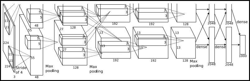
• 위 아키텍처 삽화에서 2가지 오탈자가 있다. 첫 번째론 입력 레이어의 입력 이미지 크기가 224로 되어 있지만 227이 되어야 한다. 두 번째론 두 번째 convolution layer에서 kernel size가 3x3이지만 5x5가 되어야 한다. 
• 전체 아키텍처에서 top/bottom으로 두 그룹으로 나뉘어 있는데 이는 GPU 2개를 병렬로 사용했기 때문이다. 
• 레이어 각각의 Input/output과 파라미터를 계산하면 다음과 같다.

 

Index	Convolution	Max Pooling	Normalization	Fully Connected
1	input: 227x227x3 output: 55x55x96 96 kernels of size 11x11x3, stride=4, padding=0	input: 55x55x96 output: 27x27x96 3x3 kernel, stride=2	input: 27x27x96 output: 27x27x96	none
2	input: 27x27x96 output: 13x13x256 256 kernels of size 5x5, stride=1, padding=2	input: 27x27x256 output: 13x13x256 3x3 kernel, stride= 2	input: 13x13x256 output: 13x13x256	none
3	input: 13x13x256 output: 13x13x384 384 kernels of size 3x3, stride=1, padding=1	none	none	none
4	input: 13x13x384 output: 13x13x256 384 kernels of size 3xq3, stride=1, padding=1	none	none	none
5	input: 13x13x384 output: 13x13x256 256 kernels of size 3x3, stride=1, padding=1	none	none	none
6	none	none	none	input: 6x6x256 output: 4096 parameter: 4096 neurons
7	none	none	none	input: 4096 output: 4096
8	none	none	none	input: 4096 output: 1000 softmax classes

 

 

 

3. 구현 목록 정리

3.1 레이어 구성 및 종류

• 5 convolution layers, max-pooling layers, 3 fully-connected layers 
  • overfitting 해결 위해 5개 convoutiona layer,  3개 fully-connected layer를 사용했다함
• Dropout
  • overfitting 방지 위해 fully-connected layer에 적용
  • 레이어 추가 위치는 1,2 번째 fully-connected layer에 적용
  • dropout rate = 0.5
• Local Response Normalization
  • $k$ = 2, $n$ = 5, $\alpha = 10^{-4}$, $\beta = 0.75$
  • 레이어 추가 위치는 1,2 번째 convolution layer 뒤에 적용
  • 적용 배경은 모델의 일반화를 돕는 것을 확인 (top-1, top-2 error율을 각각 1.4%, 1.2% 감소)
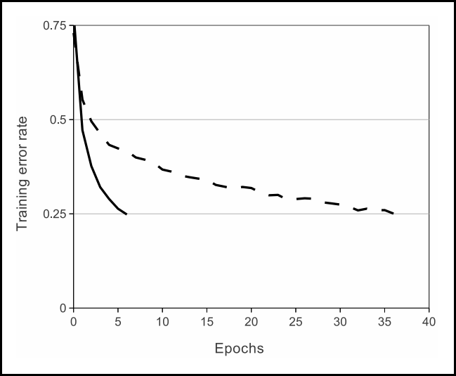
• Activation Function
  • ReLU를 모든 convolution layer와 fully-connected에 적용
  • 적용 배경은 아래 그래프처럼 실선인 ReLU가 점선인 tanH보다 빠르게 학습했음

 

2. 하이퍼 파라미터

• optimizer: SGD
• momentum: 0.9
• weight decay: 5e-4
• batch size: 128
• learning rate: 0.01
• adjust learning rate: validation error가 현재 lr로 더 이상 개선 안되면 lr을 10으로 나눠줌. 0.01을 lr 초기 값으로 총 3번 줄어듦
• epoch: 90

그리고 별도로 레이어에 가중치 초기화를 진행 해줌

• 편차를 0.01로 하는 zero-mean 가우시안 정규 분포를 모든 레이어의 weight를 초기화
• neuron bias: 2, 4, 5번째 convolution 레이어와 fully-connected 레이어에 상수 1로 적용하고 이외 레이어는 0을 적용.

def _init_bias(self):
    for layer in self.layers:
        if isinstance(layer, nn.Conv2d):
            nn.init.normal_(layer.weight, mean=0, std=0.01)
            nn.init.constant_(layer.bias, 0)

    nn.init.constant_(self.layers[4].bias, 1)
    nn.init.constant_(self.layers[10].bias, 1)
    nn.init.constant_(self.layers[12].bias, 1)
    nn.init.constant_(self.classifier[1].bias, 1)
    nn.init.constant_(self.classifier[4].bias, 1)
    nn.init.constant_(self.classifier[6].bias, 1)

참고로 헷갈렸던 것은 위 nn.init.constant_(layer.bias, 0)에서의 0은 bool로 편향 존재 여부를 나타내는 것이지 bias를 0으로 설정하는 것이 아니다. 

 

3. 이미지 전처리

• 고화질 이미지를 256x256 사이즈로 다운 샘플링후 이미지의 center에서 cropped out
• 각 픽셀에서 training set에 대한 평균 값을 빼줌

 

이를 바탕으로 전체 코드를 구현하면 아래와 같다. 크게 나누어 보자면 5가지 정도가 될 수 있다.

1. 레이어 구성 2. 가중치 초기화 3. 하이퍼파라미터 설정 4. 이미지 전처리 5. 학습 로직 작성이다. 참고로 이미지 전처리에 사용하는 transform 메서드에서 사용되는 상수 값은 별도로 논문에 기재되어 있지 않기에 pytorch 공식 documentation에서 기본 값을 가져와서 사용했다.

import os
import torch
import torch.nn as nn
import torch.nn.functional as F
import torch.optim
import torchvision.datasets as datasets
import torchvision.transforms as transforms
from torch.utils import data
import logging
from glob import glob

logging.basicConfig(level=logging.INFO)
class AlexNet(nn.Module):
    def __init__(self, num_classes=1000):
        super().__init__()
        self.num_classes = num_classes
        print (f"[*] Num of Classes: {self.num_classes}")
        self.layers = nn.Sequential(
            nn.Conv2d(kernel_size=11, in_channels=3, out_channels=96, stride=4, padding=0),
            nn.ReLU(), # inplace=True mean it will modify input. effect of this action is reducing memory usage. but it removes input.
            nn.LocalResponseNorm(alpha=1e-3, beta=0.75, k=2, size=5),
            nn.MaxPool2d(kernel_size=3, stride=2),
            nn.Conv2d(kernel_size=5, in_channels=96, out_channels=256, padding=2, stride=1),
            nn.ReLU(),
            nn.LocalResponseNorm(alpha=1e-3, beta=0.75, k=2, size=5),
            nn.MaxPool2d(kernel_size=3, stride=2),
            nn.Conv2d(kernel_size=3, in_channels=256, out_channels=384, padding=1, stride=1),
            nn.ReLU(),
            nn.Conv2d(kernel_size=3, in_channels=384, out_channels=384, stride=1, padding=1),
            nn.ReLU(),
            nn.Conv2d(kernel_size=3, in_channels=384, out_channels=256, stride=1, padding=1),
            nn.ReLU(),
            nn.MaxPool2d(kernel_size=3, stride=2))
        self.avgpool = nn.AvgPool2d((6, 6))
        self.classifier = nn.Sequential(
            nn.Dropout(p=0.5),
            nn.Linear(in_features=256, out_features=4096),
            nn.ReLU(),
            nn.Dropout(p=0.5),
            nn.Linear(in_features=4096, out_features=4096),
            nn.ReLU(),
            nn.Linear(in_features=4096, out_features=self.num_classes))

        self._init_bias()


    def _init_bias(self):
        for layer in self.layers:
            if isinstance(layer, nn.Conv2d):
                nn.init.normal_(layer.weight, mean=0, std=0.01)
                nn.init.constant_(layer.bias, 0)

        nn.init.constant_(self.layers[4].bias, 1)
        nn.init.constant_(self.layers[10].bias, 1)
        nn.init.constant_(self.layers[12].bias, 1)
        nn.init.constant_(self.classifier[1].bias, 1)
        nn.init.constant_(self.classifier[4].bias, 1)
        nn.init.constant_(self.classifier[6].bias, 1)


    def forward(self, x: torch.Tensor) -> torch.Tensor:
        x = self.layers(x)
        x = self.avgpool(x)
        x = torch.flatten(x, 1) # 1차원화
        x = self.classifier(x)
        return x


if __name__ == "__main__":
    seed = torch.initial_seed()
    print (f'[*] Seed : {seed}')
    NUM_EPOCHS = 1000 # 90
    BATCH_SIZE = 128
    NUM_CLASSES = 1000
    LEARNING_RATE = 0.01
    IMAGE_SIZE = 227
    TRAIN_IMG_DIR = "C:/github/paper-implementation/data/ILSVRC2012_img_train/"
    #VALID_IMG_DIR = "<INPUT VALID IMAGE DIR>"
    CHECKPOINT_PATH = "./checkpoint/"

    device = torch.device('cuda' if torch.cuda.is_available() else 'cpu')
    print (f'[*] Device : {device}')

    alexnet = AlexNet(num_classes=NUM_CLASSES).cuda()
    checkpoints = glob(CHECKPOINT_PATH+'*.pth') # Is there a checkpoint file?
    if checkpoints:
        checkpoint = torch.load(checkpoints[-1])
        alexnet.load_state_dict(checkpoint['model'])
    #alexnet = torch.nn.parallel.DataParallel(alexnet, device_ids=[0,]) # for distributed training using multi-gpu

    transform = transforms.Compose(
        [transforms.CenterCrop(IMAGE_SIZE),
         transforms.RandomHorizontalFlip(),
         transforms.ToTensor(),
         transforms.Normalize(mean=[0.485, 0.456, 0.406], std=[0.229, 0.224, 0.225]),
        ])
        
    train_dataset = datasets.ImageFolder(TRAIN_IMG_DIR, transform=transform)
    print ('[*] Dataset Created')

    train_dataloader = data.DataLoader(
        train_dataset,
        shuffle=True,
        pin_memory=False, # more training speed but more memory
        num_workers=8,
        drop_last=True,
        batch_size=BATCH_SIZE
    )
    print ('[*] DataLoader Created')

    optimizer = torch.optim.SGD(momentum=0.9, weight_decay=5e-4, params=alexnet.parameters(), lr=LEARNING_RATE) # SGD used in original paper
    print ('[*] Optimizer Created')

    lr_scheduler = torch.optim.lr_scheduler.ReduceLROnPlateau(optimizer=optimizer, factor=0.1, verbose=True, patience=4) # used if valid error doesn't improve.
    print ('[*] Learning Scheduler Created')

    steps = 1
    for epoch in range(50, NUM_EPOCHS):
        logging.info(f" training on epoch {epoch}...")        
        for batch_idx, (images, classes) in enumerate(train_dataloader):
            images, classes = images.cuda(), classes.cuda()
            output = alexnet(images)
            loss = F.cross_entropy(input=output, target=classes)
            optimizer.zero_grad()
            loss.backward()
            optimizer.step()
            if steps % 50 == 0:
                with torch.no_grad():
                    _, preds = torch.max(output, 1)
                    accuracy = torch.sum(preds == classes)
                    print ('[*] Epoch: {} \tStep: {}\tLoss: {:.4f} \tAccuracy: {}'.format(epoch+1, steps, loss.item(), accuracy.item() / BATCH_SIZE))
            steps = steps + 1

        lr_scheduler.step(metrics=loss)

        if epoch % 5 == 0:
            checkpoint_path = os.path.join(CHECKPOINT_PATH, "model_{}.pth".format(epoch))
            state = {
                'epoch': epoch,
                'optimizer': optimizer.state_dict(),
                'model': alexnet.state_dict(),
                'seed': seed
            }
            torch.save(state, checkpoint_path)

 

AlexNet의 경우 비교적 구현이 어렵지 않은 편이기에 논문 구현을 연습하기에 좋다고 느낀다.

 

Code: https://github.com/roytravel/paper-implementation

 

Reference

[1] https://github.com/YOUSIKI/PyTorch-AlexNet/blob/de241e90d3cb6bd3f8c94f88cf4430cdaf1e0b55/main.py

[2] https://github.com/Ti-Oluwanimi/Neural-Network-Classification-Algorithms/blob/main/AlexNet.ipynb

[3] https://github.com/daeunni/CNN_PyTorch-codes/blob/main/AlexNet(2012).ipynb

[4] https://deep-learning-study.tistory.com/376